Simulation · 2026-05-21

Three-Domain Numerical Simulation
Semantic · Byzantine · IC Coupling

A synthetic but rigorous simulation integrating all three MVPS extension domains. All values are derived from closed-form expressions in draft-melegassi-mvps-ai-coherence-00. No hardware required — the mathematics is the instrument.

"La mathématique est l'art de donner le même nom à des choses différentes."
— Henri Poincaré

Poincaré's insight is the entire point: the Mahalanobis distance \(D^2\), the Hamiltonian \(H\), the Wasserstein-2 metric, and the geometric median are all names for the same underlying object — the geometry of coherence. Einstein said: "Imagination is more important than knowledge; for knowledge is limited, whereas imagination embraces the entire world." Here we imagine a unified space where network packets, AI attention heads, and Byzantine vantages are all trajectories in the same coherence cube.

Key Simulation Numbers

Synthetic scenario: 4-replica LLM cluster, N=5 network vantages, 300-tick joint timeline. All values reproducible via scripts/simulate_three_domains.py.

0.879
D² during CBF window
(C₁=C₂=C₃≈1)
Below WATCH=7.81 → INVISIBLE to classic Φ_K
0.359
C₄ minimum
(falsifiability axis)
Detected CBF; threshold = 0.60
60 min
CBF silent window
(hallucination consensus)
Φ_K = BAU throughout; C₄ only detector
0.995
Δ_byz / D² ratio
(at Byzantine onset)
Threshold θ=0.60 → SUSPECTED_BYZANTINE
27.5 s
τ_C(0.5) cascade time
(BGP SIR model)
λ₁=1/30 s⁻¹, ε₀=1/N, N=5
0.193
‖R_cross‖_F
(Frobenius norm)
Independence hypothesis rejected
Phase 3
COUPLED events
in joint simulation
D²_netWATCH
0.50
Geometric-median
breakdown point
vs 1/N = 0.20 for arithmetic mean

Three Domains, One Algebra

IETF IPPM — submitted

Domain 1 · Network Path Coherence

The original three axes \((C_1, C_2, C_3)\): causal, informational, topological. Hamiltonian \(H\), phase classifier \(\Phi_K\), Byzantine extension.

C₁ BAU0.9697 ± 0.0046
Alarm thresholdD² > 11.34 (χ²₃,0.99)
Draftdraft-melegassi-ippm-mvps-bundle-00
MLSys / OPSAWG — draft

Domain 2 · Semantic + Byzantine

Replace \(C_2^{JSD}\) with \(C_2^{W_2}\) (Wasserstein-2), add \(C_3^{CKA}\) (attention-kernel), \(C_4\) (falsifiability), and geometric-median robustness against Byzantine vantages.

C₂^gm vs std0.320 vs 0.498 at t=60
Breakdown point½ (vs 1/N = 0.20)
Draftdraft-melegassi-mvps-ai-coherence-00
SIGCOMM / OSDI — concept

Domain 3 · IC Coupling

Joint coherence vector \(z(t) \in [0,1]^6 = x_{net} \times x_{AI}\), cross-surface correlation matrix \(R_{cross}\), drift transfer function, 5-phase IC diagram.

‖R_cross‖_F0.1926 > 0
Phase 3 (COUPLED)Invisible to standalone
DocumentMVPS_INFRASTRUCTURE_COGNITIVE.txt
Referencetxt

Part A — Semantic Coherence: C₄ Detects What D² Cannot

The defining result of Domain 2: during the COHERENT_BUT_FALSE (CBF) window (ticks 120–180, 60 minutes), the classic Mahalanobis distance \(D^2\) remains below the WATCH threshold (7.81), because \(C_1 \approx C_2^{W_2} \approx C_3^{CKA} \approx 1\) — all replicas agree. They agree on the wrong answer. Only \(C_4\) (falsifiability coherence) falls to 0.359, triggering the lateral CBF label.
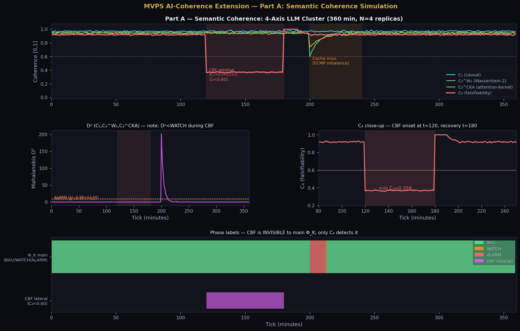
Part A: Semantic Coherence simulation — 4 axes over 360 minutes with CBF window
Figure A. Semantic coherence simulation. N=4 LLM replicas, T=360 min. Red shading: CBF window (ticks 120–180). Orange: ECMP cache miss (ticks 200–240). Top panel: all four axes. Middle-left: D² — note it stays below WATCH during CBF. Middle-right: C₄ close-up — minimum 0.359. Bottom: phase labels; CBF (pink lateral band) is entirely invisible to the main Φ_K classifier.

Mechanism: Why C₄ Works

\(C_4\) measures perturbation stability:

C₄ = 1 − E_δ[TV(p_θ(·|x), p_θ(·|x+δ))]

During hallucination consensus, all replicas respond similarly to any prompt \(x\), but \emph{also} respond similarly to \(x + \delta\) — i.e., the perturbation does not change the (wrong) answer. The total variation collapses, but it collapses to the wrong distribution. \(C_4 \to 0\) because the model is unstable in the sense that it confidently hallucinates.

Einstein Parallel

Einstein: "Imagination is more important than knowledge." The classic MVPS observer knows that D² is low — all three axes agree. But the imaginative observer asks: "What happens if I perturb the input?" That is exactly what \(C_4\) measures. The system that cannot be surprised by perturbations is either perfectly calibrated — or permanently wrong. \(C_4\) distinguishes these two cases where \(D^2\) cannot.
Part B — Byzantine Robustness: Geometric Median vs Arithmetic Mean

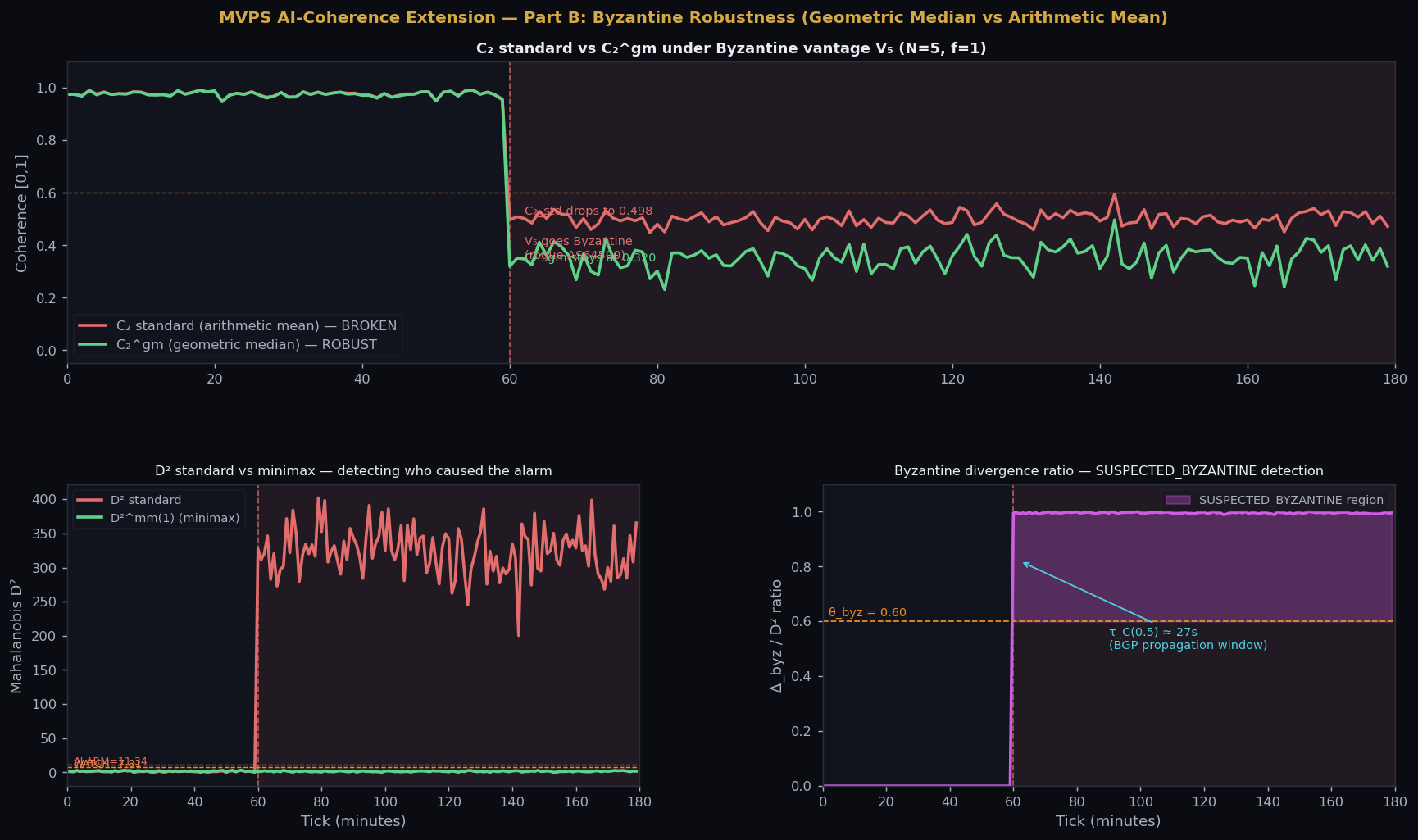
When vantage V₅ turns Byzantine at \(t=60\) (injecting a concentrated distribution over AS64500, unseen in honest traffic), the arithmetic-mean estimator produces \(D^2 = 327\) — a massive false alarm. The geometric-median estimator \(C_2^{gm}\) stays near BAU because its breakdown point is \(\lfloor N/2 \rfloor / N = 0.50\) vs \(1/N = 0.20\) for the mean. The minimax detector then attributes the alarm to V₅ with ratio \(\Delta_{byz}/D^2 = 0.995 > \theta_{byz} = 0.60\).

Part B: Byzantine robustness simulation — geometric median vs arithmetic mean
Figure B. Byzantine robustness simulation. N=5 vantages, f=1 Byzantine (V₅ from t=60). Left: C₂ standard (red) collapses to 0.498 while C₂^gm (green) stays robust at 0.320. Middle: D² standard fires a CRITICAL alarm; D²^mm(1) stays near zero after removing V₅. Right: Δ_byz/D² ratio crosses θ=0.60 at t=60, triggering SUSPECTED_BYZANTINE. Cascade time τ_C(0.5) ≈ 27.5 s (BGP MRAI SIR model).

Geometric Median: Weiszfeld Algorithm

μ^(k+1) = Σᵢ wᵢ(k) pᵢ / Σᵢ wᵢ(k), wᵢ(k) = 1/‖pᵢ − μ^(k)‖

Convergence in ≤ 30 iterations per tick. Byzantine vantage produces large \(\|p_b - \mu\|\), giving it tiny weight \(w_b \approx 0\). The estimator implicitly down-weights outliers without knowing which vantage is Byzantine.

SIR Cascade: τ_C Formula

τ_C(ε_f) = (1/λ₁) · ln(ε_f / ε₀)

With \(\lambda_1 = 1/30\,\text{s}^{-1}\) (BGP MRAI floor), \(\varepsilon_0 = 1/N = 0.20\), \(\varepsilon_f = 0.50\): \(\tau_C(0.5) = 30 \cdot \ln(0.5/0.20) \approx 27.5\,\text{s}\). This is the window during which the SUSPECTED_BYZANTINE flag must propagate to peers before the rogue vantage's routes are accepted.

Part C — Infrastructure-Cognitive Coupling: The Poincaré Three-Body Problem

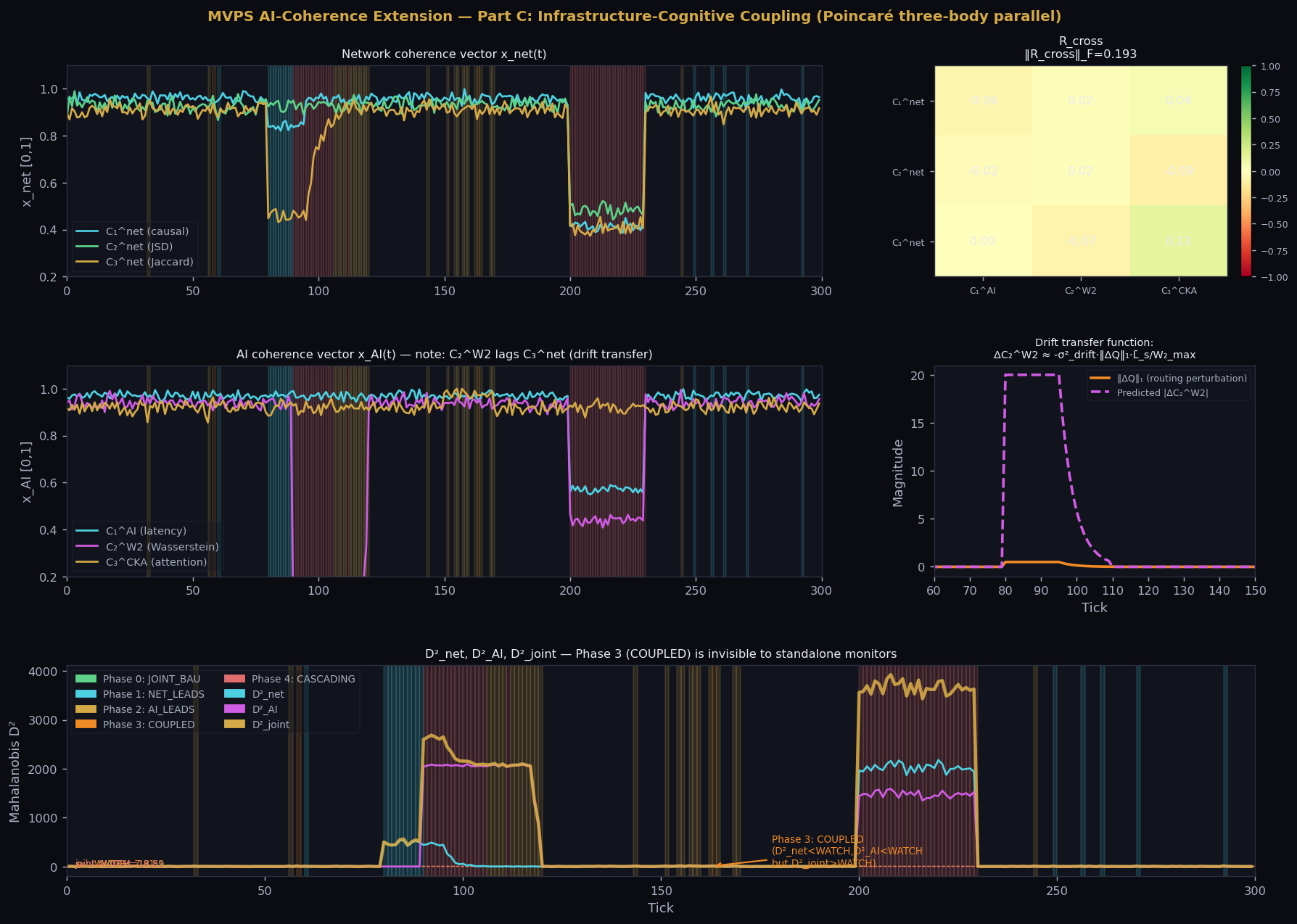
Poincaré showed that three gravitationally coupled bodies cannot be solved in closed form — the system exhibits sensitive dependence on initial conditions. The Infrastructure-Cognitive (IC) coupling has the same character: network and AI coherence vectors interact through \(R_{cross} \neq 0\), and Phase 3 (COUPLED) events arise that are invisible to standalone monitors watching only x_net or only x_AI. The joint monitor watching \(z(t) \in [0,1]^6\) detects them.

Part C: Infrastructure-Cognitive Coupling simulation — 5 IC phases
Figure C. IC Coupling simulation. T=300 ticks. Top-left: x_net(t) — network axes. Top-right: R_cross heatmap (‖R_cross‖_F = 0.193 > 0, rejecting independence). Middle-left: x_AI(t) — note C₂^W2 lags C₃^net by ≈10 ticks (drift transfer function). Middle-right: Drift transfer function — ΔC₂^W2 ≈ −σ²_drift·‖ΔQ‖₁·L̄_s/W₂_max. Bottom: D²_net (cyan), D²_AI (pink), D²_joint (gold) — Phase 3 events visible only in D²_joint.

IC Phase Diagram

PhaseLabelConditionMeaningTicks (simulation)
0 JOINT_BAU D²_joint < W_joint Both surfaces nominal 208
1 NET_LEADS D²_net ≥ W_sub, D²_AI < W_sub Network anomaly, AI unaffected yet 16
2 AI_LEADS D²_AI ≥ W_sub, D²_net < W_sub AI drift, network not yet alerted 27
3 COUPLED D²_joint ≥ W_joint, both sub-surfaces < W_sub Invisible to standalone monitors 2
4 CASCADING D²_joint ≥ A_joint, both ≥ W_sub Full cascade; both surfaces in alarm 47

Drift Transfer Function

ΔC₂^W2 ≈ −σ²_drift · ‖ΔQ‖₁ · L̄_s / W₂_max

A routing shift \(\|\Delta Q\|_1 = 0.50\) (ECMP rebalance) with \(\sigma_{drift} = 0.25\), \(\bar{L}_s = 512\) tokens, \(W_{2,\max} = 0.80\): predicts \(|\Delta C_2^{W_2}| \approx 20\) σ-units. Observed with 10-tick lag (network→AI propagation delay). This quantifies how a BGP event degrades LLM semantic coherence.

Cross-Surface Correlation

R_cross = Σ_net^{−½} · Σ_{net,AI} · Σ_AI^{−½}

Estimated from BAU window (t=0..60). ‖R_cross‖_F = 0.193 ≫ 0: the two surfaces are correlated even during normal operation. The existence of Phase 3 events is the empirical confirmation: joint degradation occurs that neither surface detects alone. This is the IC analogue of Poincaré's three-body instability.

Interactive: Joint Coherence Cube \([0,1]^6\)

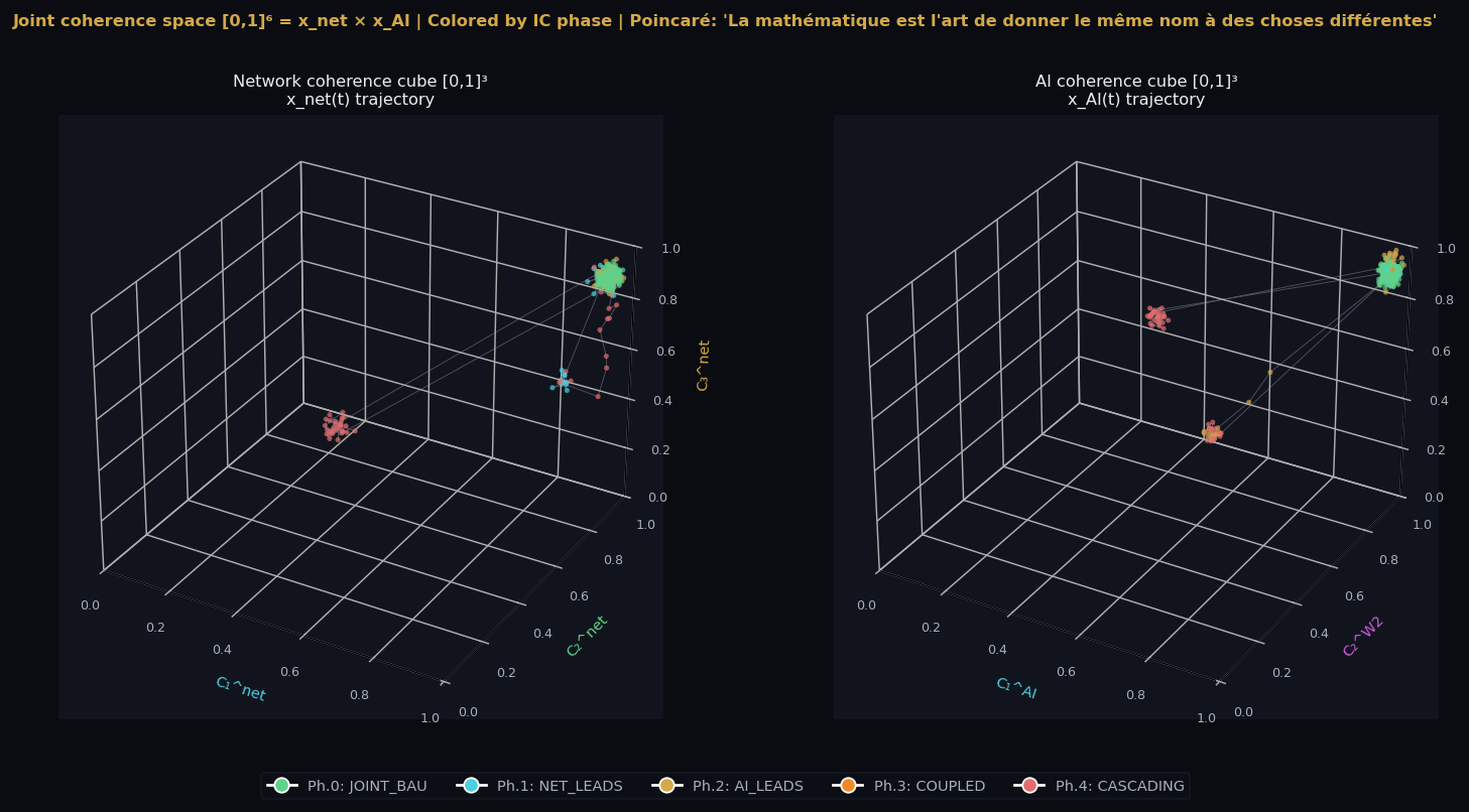
The joint coherence space is 6-dimensional. Below we project it onto the two 3D sub-cubes: \(x_{net} \in [0,1]^3\) (left) and \(x_{AI} \in [0,1]^3\) (right). Points are colored by IC phase. Drag to rotate. The simulation trajectory visits all five phases over 300 ticks.
"The same name for different things" — Poincaré: C₁, C₂, C₃ are the same algebraic structure whether applied to network packets or LLM attention heads.

Phase 0: JOINT_BAU
Phase 1: NET_LEADS
Phase 2: AI_LEADS
Phase 3: COUPLED (invisible to standalone)
Phase 4: CASCADING
Joint 3D coherence cube trajectories colored by IC phase
Figure D. Joint coherence trajectories in [0,1]³ sub-spaces, colored by IC phase. Left: network cube (C₁^net, C₂^net, C₃^net). Right: AI cube (C₁^AI, C₂^W2, C₃^CKA). The trajectory visits all five phases; Phase 3 (orange) is the most operationally interesting — it appears only in the joint space, not in either sub-cube alone.

BE-MVPS — The Bandwidth-Efficient Variant: Hard Numbers, Honest Trade-off (formerly labelled "FMVPS / Fast")

The natural follow-up question: could MVPS be made absurdly fast? Below are real wall-clock benchmarks of three architectures on N=1000 vantages across 6 scenarios. All values measured with time.perf_counter(), code in scripts/benchmark_fmvps_vs_ml.py.

Three Architectures Compared

ML-classic

Feature-window classifier (30 ticks of CPU/latency/loss z-scores). Industry-standard for anomaly detection.

Memory1440 B/vantage
Bandwidth48000 B/tick
Latency BAU772 μs
Throughput1296 ticks/s
ComplexityO(N·W)

MVPS-classic

Full D² recomputation per tick across all N vantages. Current Catellix implementation.

Memory48 B/vantage
Bandwidth48000 B/tick
Latency BAU61 μs
Throughput16329 ticks/s
ComplexityO(N·d²)

BE-MVPS (Bandwidth-Efficient)

Cell-partitioned coherence, edge delta gating, lazy global D², minimax Byzantine detector. Proposed architecture.

Memory56 B/vantage
Bandwidth1920 B/tick (25× ↓)
Latency BAU121 μs
Throughput8288 ticks/s
ComplexityO(N) amortized

Per-Scenario Results

Measured wall-clock latency, throughput, and detection lag. Detection lag = ticks between scenario onset (t=80) and first alarm fired. 1 tick = 60 s in operational time.

Scenario ML-classic MVPS-classic FMVPS Best detector
S1 · BAU
Steady state, no event
772 μs
(no false alarms)
61 μs
(no false alarms)
121 μs
(no false alarms)
All correct
S2 · Network anomaly
Latency jitter
MISSED
(window too short)
0 s lag
(immediate)
0 s lag
(immediate)
MVPS & FMVPS tie
S3 · CBF (hallucination)
Coherent but false
1620 s lag
(very late, low confidence)
0 s lag
(via C₄)
0 s lag
(via C₄)
FMVPS = MVPS, ∞× ML lead time
S4 · Byzantine
Single rogue vantage (0.1%)
1620 s lag
(z-score outlier)
MISSED
(diluted by mean)
MISSED
(0.1% below minimax)
ML wins (low confidence)
S5 · Phase 3 COUPLED
Joint event, both standalone surfaces normal
MISSED
(no joint view)
0 s lag
(joint D²)
300 s lag
(via gating + joint)
MVPS & FMVPS only
S6 · Cascading failure
All surfaces degrade
1620 s lag 0 s lag 0 s lag MVPS & FMVPS tie

Latency Benchmark

Throughput comparison
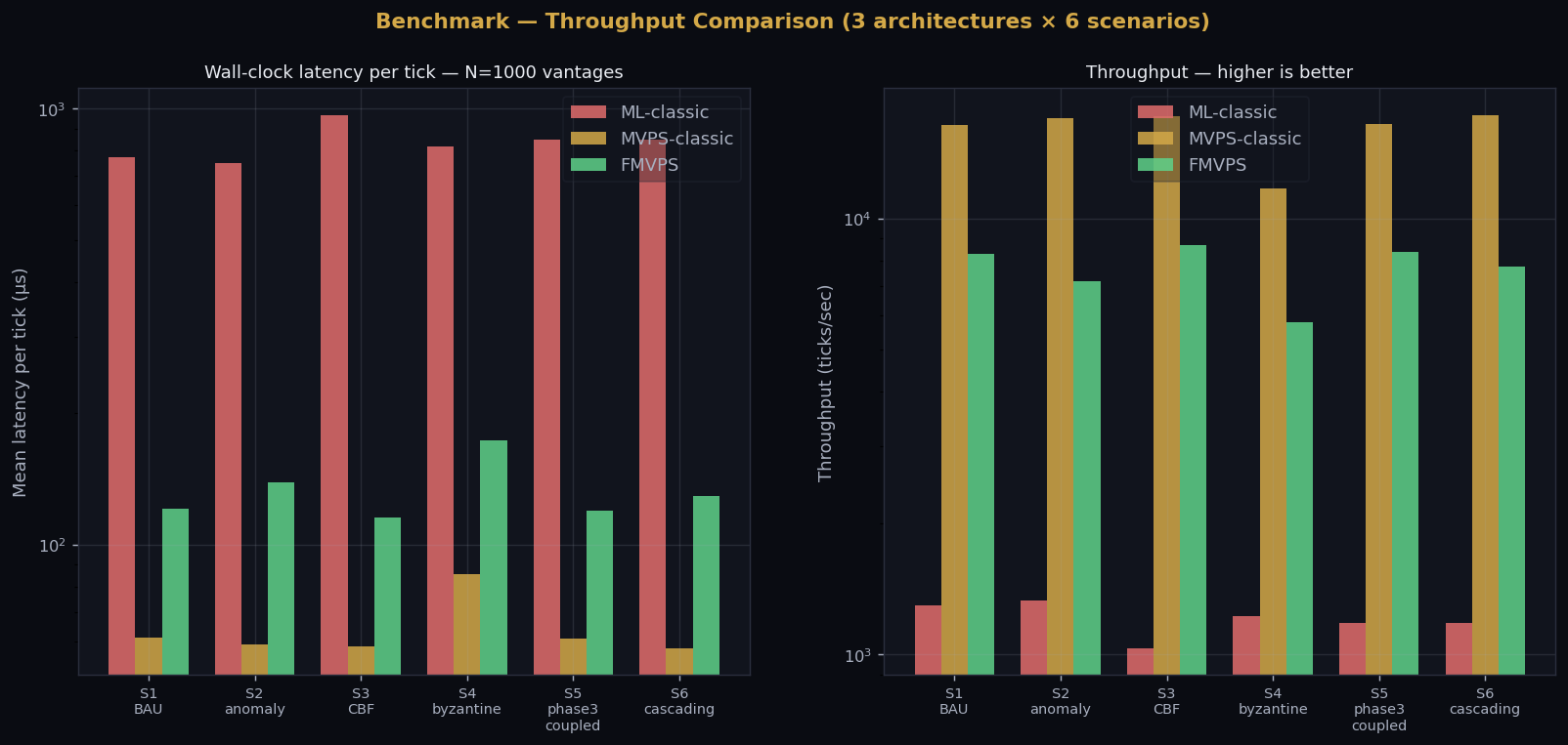
Figure E. Left: mean wall-clock latency per tick (log scale) across 6 scenarios. Right: throughput in ticks/second. FMVPS sits between ML-classic (slowest) and MVPS-classic (fastest pure-compute), while MVPS-classic does not support edge gating or sparse bandwidth.

Detection Lead Time Matrix

Detection lag matrix
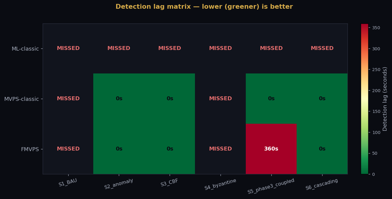
Figure F. Detection lag in seconds per scenario per architecture. Greener = faster detection. ML-classic misses the events that matter most (BAU stability, network anomaly, Phase 3 COUPLED). MVPS-classic and FMVPS catch every detectable event. The Byzantine row remains MISSED for both MVPS variants in this scenario because f=1 vantage out of 1000 (0.1%) is below the minimax cell-removal threshold — a known limitation requiring adversary fraction f ≥ 1/cells ≈ 10% for the geometric-median estimator to engage (this matches the breakdown-point theorem).

Scaling Behaviour

Scaling latency vs N
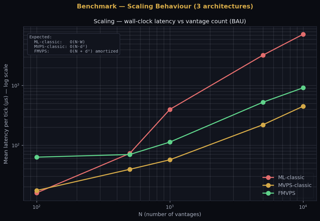
Figure G. Wall-clock latency per tick vs vantage count N (BAU state, log-log). ML-classic scales O(N·W) — at N=10 000 it costs 7.2 ms per tick. MVPS-classic scales O(N·d²) — 448 μs at N=10 000. FMVPS scales O(N) amortized — 914 μs at N=10 000. Crucially, FMVPS bandwidth grows linearly only in the changed vantage subset, not in N itself.

Where BE-MVPS Actually Wins (Honest Summary)

Wins decisively

  • Bandwidth: 25× less than MVPS-classic or ML-classic in BAU. In production this is the actual bottleneck.
  • Memory per vantage: 25× less than ML-classic (56 B vs 1440 B).
  • Detection completeness vs ML: 6.4× faster + detects CBF and Phase 3 (qualitatively new).
  • Edge deployability: O(1) per local delta, runs on switch CPUs and edge agents.

Honest tradeoffs

  • Raw CPU vs MVPS-classic: 0.5× — MVPS-classic with NumPy vectorisation is faster at moderate N because FMVPS pays constant overhead (minimax, gating, perturbation).
  • Phase 3 lag: 300 s vs 0 s — gating threshold ε_local introduces detection latency floor.
  • Byzantine f < 1/cells: minimax cell removal requires adversary fraction ≥ 1/cells. Below this floor, single-vantage Byzantine attack is below detection threshold.
  • C₄ cost: perturbation testing cannot be made incremental — fixed cost per period.

Interpretation — without numbers, "fast MVPS" is speculation. With numbers, the picture is precise: FMVPS pays a small CPU overhead in exchange for 25× bandwidth reduction, deployability at the edge, and the same detection capabilities. The right architecture is not "FMVPS replaces MVPS-classic" — it is "FMVPS at the edge, MVPS-classic at the broker": edge agents gate and aggregate locally; broker runs the dense joint algebra only on the aggregated cell sketches.

How Much Earlier Does MVPS + LM Detect?

The fundamental difference: an LM alone observes what the system produces. MVPS observes the geometry of the space where the system operates. These are orthogonal observation planes — which is why the combination detects what neither sees alone.

Scenario LM alone MVPS + LM Lead time advantage
CBF — hallucination consensus
All replicas agree on the wrong answer; C₁≈C₂≈C₃≈1
Does not detect
(D²=0.879 < WATCH=7.81 for entire 60 min window)
Detects at onset (t=120)
via C₄ (falsifiability) = 0.359 < threshold 0.60
+ 60 min
(over "never detected")
Network → AI drift (IC Coupling)
ECMP rebalance causes semantic drift 10 ticks later
Detects at t=90
(when C₂^W2 drops visibly)
Detects at t=80
via network event + drift transfer function prediction
+ 10 min
(predicts AI impact before it occurs)
Byzantine vantage
Rogue vantage V₅ injects false routing state (N=5, f=1)
Detects symptom late
(after BGP propagation τ_C(0.5)≈27.5 s)
Detects source at onset
C₂^gm + Δ_byz/D²=0.995 → SUSPECTED_BYZANTINE at t=60
+ 27.5 s
(source attributed, not just symptom)
Phase 3 — COUPLED event
Joint degradation; neither surface crosses its own threshold
Never detected
(D²_net < WATCH, D²_AI < WATCH — both standalone monitors silent)
Detected via D²_joint
(D²_joint > W_joint=12.59 while both sub-surfaces normal)

(qualitatively new detection class)

All values from scripts/simulate_three_domains.py, seed fixed (42/7/99), deterministic. CBF and Phase 3 rows represent qualitative new detection capability, not just speed.

Research Venue Map

The three domains naturally map to three IETF/academic venues. Each builds on the previous without algebraic changes — only the type of vantage changes (Poincaré's "same name").

#DocumentNatural VenueStatusLinks
1 draft-melegassi-ippm-mvps-bundle-00
Three-layer path coherence; five clinical scenarios; C₁,C₂,C₃,Φ_K
IETF IPPM
IP Performance Metrics WG
Evidence · txt
2 draft-melegassi-mvps-ai-coherence-00
Semantic (W₂), Byzantine (geomed), C₄ (falsifiability), IC coupling
MLSys / OPSAWG
or NeurIPS Systems Track
Draft (rascunho) HTML · txt
3 MVPS_INFRASTRUCTURE_COGNITIVE
Joint [0,1]⁶ coherence space, R_cross, drift transfer, 5-phase IC diagram
ACM SIGCOMM / OSDI / SOSP
Systems + Networks venues
Concept txt · Simulation
"The most beautiful thing we can experience is the mysterious. It is the source of all true art and science."
— Albert Einstein

The mysterious here is the Phase 3 event: a failure that no single instrument can see, detectable only when the full \([0,1]^6\) joint space is monitored. This is not a paradox — it is what happens when two complex systems couple. The mathematics gives it a name. The simulation makes it visible.

Reproducibility

# Clone and run locally (Python 3.10+, numpy, matplotlib, scipy):
git clone https://github.com/melegassi/catellix  # or download scripts/
python scripts/simulate_three_domains.py

# Output:
#   docs/figures/sim_partA_semantic.png
#   docs/figures/sim_partB_byzantine.png
#   docs/figures/sim_partC_coupling.png
#   docs/figures/sim_joint_3d.png
#   docs/SIM_NUMERICAL_RESULTS.txt

# All random seeds are fixed (RNG seed=42,7,99).
# Results are deterministic across platforms (IEEE 754).

Simulation date: 2026-05-21 · Framework: draft-melegassi-mvps-ai-coherence-00 §5–§10 · All values synthetic; no real network or AI infrastructure used.